Learnings from Molecular Dynamic Simulation

Introduction

To understand the process of creating and running a molecular dynamic simulation using NAMD and VMD, I ran a simple simulation of a water box. The first half of the post discusses MD Simulations and their sophistication and intricacies. The second half discusses creating and simulating a water box using a high-performance computing cluster.

Computer Simulations

Computer simulations help us better analyze the properties of molecular assemblies in terms of microscopic interactions and structure of the same. This works as a supplement to traditional experiments, empowering us to learn something new that we couldn’t learn any other way. Molecular dynamics (MD) and Monte Carlo are the most common simulation techniques (MC). Computer simulations help link time scales and the microscopic length with the macroscopic world in the laboratory. It provides a view of the interactions among molecules and obtains accurate predictions of the bulk properties. Molecular dynamics (MD) is a procedure where the motion of the particles of a system over a specific period is recorded by solving Newton’s equations of motion. This is done for each particle in the system over the simulation duration. However, the MD simulation method was introduced in the 1950s by Marshall Rosenbluth and Nicholas Metropolis in the form of the Metropolis-Hastings algorithm.


The general procedure for MD Simulation is illustrated

NAMD

NAMD was first introduced by Nelson et al., who was part of the theoretical biophysics group, in the year 1995. It was implemented and created using C++. Currently, the theoretical biophysics group and the parallel programming laboratory at the University of Illinois develop, upgrade, and maintain NAMD. NAMD is used to perform dynamic molecular simulations. For any simulation, the input files required and their description are given below.

PDB (Protein Data Bank) - Contains information on the coordinates of atoms of the Protein
PSF (Protein Structure File) - Contains all the information necessary to convert a list of residual names into a complete PSF structure file. Aids with the automatic designation of hydrogen atoms to the protein
Topology file - Contains all the molecular-specific information needed to apply a particular force field to the molecular system
Parameter file - Contains all the numerical constants necessary to evaluate energies, forces, speed, and position of the atoms of the protein

VMD

The theoretical and computational biophysics group established VMD under the supervision of Klaus Schulten. VMD has Tcl (a high-level programming language) and Python interpreters. VMD is used along with NAMD to visualize the proteins and the steps involved in the simulation. The theoretical and computational biophysics group currently maintains it. VMD recognizes various files of molecular data for visualization purposes. The list below gives more information about the same.

Protein Data Bank files
X-PLOR and Chemistry at Harvard Macromolecular Mechanics (CHARMM) PSF files
X-PLOR and Chemistry at Harvard Macromolecular Mechanics (CHARMM) trajectory DCD files
X-PLOR and Chemistry at Harvard Macromolecular Mechanics (CHARMM) trajectory DCD files
Assisted Model Building with Energy Refinement (AMBER) trajectory and structure files
GROningen MAchine for Chemical Simulations (GROMACS) trajectory and structure files

Molecular Dynamics Simulation

Characteristics of Molecular Dynamic Simulation include the following:

It is a deterministic technique
It only takes into consideration the the intermolecular forces and the starting position of each particle in the system
It can be successfully be used as a statistical mechanics method
The data recorded about the distances and the velocities can be averaged over time and over all the molecules of the system to obtain the thermodynamic quantities of the system
It provides atomic and molecular level information on the system


The Steps Involved in Molecular Dynamic Simulation

The main disadvantage of Molecular Dynamic Simulation is that the result is often an approximate measure because solving the Schrodinger equation to obtain the wavefunction that accurately describes atom/particle is computationally expensive and time-consuming. However, the error obtained from simulation can be minimized by choosing the correct potential function. A wide range of potential functions makes the simulation results realistic and more precise.

The Algorithm

Newton’s equation of motions are solved for all the system particles for all molecular dynamic simulations.

As input we need only the following:

The starting set of coordinates of the atoms of a system.
The set of potential functions for obtaining the forces among various atoms/particles of the system.

The five quintessential components for any Molecular Dynamic Simulation are initial condition, boundary condition, integrator/ensemble, force calculation, and property calculation. The distinct properties calculated include - dynamic structure factor and thermal conductivity, the viscosity of the system particles, internal energy, free energy, enthalpy, and many more. The various potentials include - the Lennard-Jones potential Coulomb–Buckingham potential.

Lennard-Jones Potential

It is an intermolecular pair potential. Among all the intermolecular pairs, researchers have extensively examined the Lennard-Jones potential.

Lennard-Jones Potential Expression

Lennard-Jones Potential Graph

Coulomb–Buckingham Potential

It is a modification of the Buckingham Potential, which was put forth by Richard Buckingham. For the application of the Buckingham potential to ionic systems, the modification was made, and hence the new potential came to be known as Coulomb-Buckingham Potential.

Coulomb–Buckingham Potential Expression

Coulomb–Buckingham Potential Graph

Water Box Simulation

The water box is modelled by utilizing the VMD software. We use the “Add Solvation Box” command to generate the water box. The command can be accessed as follows:

VMD > Extensions > Modeling > Add Solvation Box

The command generates the PDB (Protein Data Bank) and the PSF (Protein Structure File) for the water box after taking in the coordinates of the box, for our case we provide 40nm as the length of our water box, centered at (0, 0, 0). The diagram below depicts the PDB of water box generated as displayed by VMD.

Water Cube

The first few lines of the PDB file for the water box:

CRYST1   40.000   40.000   40.000  90.00  90.00  90.00 P 1           1
ATOM      1  OH2 TIP3W   5     -16.332  -9.918  -4.096  1.00  0.00      WT1  O
ATOM      2  H1  TIP3W   5     -16.776  -9.549  -4.899  1.00  0.00      WT1  H
ATOM      3  H2  TIP3W   5     -16.908  -9.621  -3.373  1.00  0.00      WT1  H
ATOM      4  OH2 TIP3W   7     -13.967 -15.124   0.891  1.00  0.00      WT1  O
ATOM      5  H1  TIP3W   7     -13.922 -14.776   1.798  1.00  0.00      WT1  H
ATOM      6  H2  TIP3W   7     -13.408 -15.912   0.961  1.00  0.00      WT1  H    

Now that the PDB and the PSF files are ready, we need to create the configuration file that NAMD uses to set parameters for the MD simulation that needs to be run. The various parameters necessary for running a simulation are - structure file, coordinate file, temperature, restartfreq, dcdfreq, xstFreq, outputEnergies, force-field parameters, cutoff, stepspercycle, timestep, langevin, langevinDamping, langevinTemp, langevinHydrogen, periodic boundary conditions, particle mesh Ewald (PME), langevinPiston, langevinPistonTarget, langevinPistonPeriod, langevinPistonDecay, langevinPistonTemp, minimize, and run.

This section explores each of these parameters in detail.

Structure - This takes as input the relative location of the structure file, in our case the PSF file generated by VMD.
```
structure       ../input/solvate.psf
```
Coordinates - Just like the structure parameter, this takes the relative location of the PDB file, which the coordinates of the structure.
```
coordinate      ../input/solvate.pdb
```
Temperature - Sets the temperature for the MD simulation (in Kelvin).
```
temperature     300
```
. Restart Frequency, DCD Frequency, XST Frequency, Output Energies - The frequency with which the restart files, DCD (coordinates), and the XST (velocity) files are generated. Output Energies rewrites the output files every fixed number of steps.
```
restartfreq     1000 # 1000 steps = 2ps
dcdfreq         1000
xstFreq         1000
outputEnergies  150
```
Force Field Parameters - paraTypeCharmm and parameters - The paraTypeCharmm parameter checks whether the parameters file is CHARMM type, and the parameter keyword takes the relative location of the force field parameter file.
```
paraTypeCharmm  on
parameters      ../input/par_all27_prot_lipid.inp
```
Cutoff - NAMD effectively removes the Van Der Waal forces of interaction by the specified cutoff value. The Fig. 2.2 illustrates the working of the Cutoff parameter.
```
cutoff          10
```
Steps per cycle - The total number of steps taken for completion of one cycle is specified by the stepspercycle parameter.
```
stepspercycle   5
```

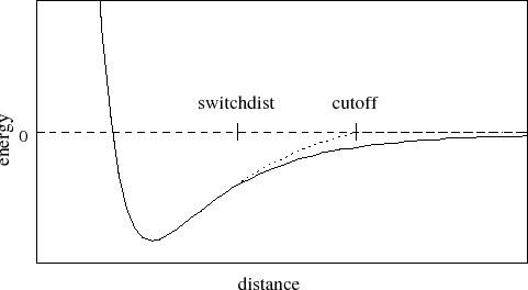
Illustration of the working of the Cutoff parameter

Time Step - The time taken to complete one step, specified in femtoseconds.
```
timestep        2.0
```
Temperature Control Parameters - The ‘langevin’ parameter specifies whether the Langevin dynamics are to be utilized. ‘langevinDamping’ specifies the damping coefficient for the said dynamics. ‘langevinTemp’ states the temperature in Kelvin for langevin dynamics. ‘langevinHydrogen’ tells NAMD whether to apply Langevin dynamics to hydrogen atoms present.
```
langevin         on
langevinDamping  1
langevinTemp     300
langevinHydrogen no
```
Periodic Boundary Conditions - The parameters cellBasisVector1, cellBasisVector2, and cellBasisVector3 state the length of the repeating units. This is implemented to avoid the finite size problem and to make the system an infinite one for smoother simulation. cellOrigin - takes as input the center/origin of the simulation.
```
cellBasisVector1 40   0   0
cellBasisVector2 0    40  0
cellBasisVector3 0    0   40
cellOrigin       0    0   0
```
Pressure Control - The ‘langevinPiston’ specifies whether the Langevin piston is to be used or not. ‘langevinPistonTarget’ specifies the target pressure required for the calculations involved in piston method, in bar. ‘langevinPistonPeriod’ specifies the duration for the piston method, in femtoseconds. ‘langevinPistonDecay’ - specifies the damping time period for the method, in femtoseconds. ‘langevinPistonTemp’ specifies the piston temperature, in Kelvin.

useGroupPressure       yes
useFlexibleCell        no
useConstantArea        no
LangevinPiston         on
LangevinPistonTarget   1.01325
LangevinPistonPeriod   100
LangevinPistonDecay    50
LangevinPistonTemp     300.0

PME or Particle Mesh Ewald is used along side with periodic boundary conditions. ‘PMEGridSpacing’ specifies the distance between the grids.

PME             yes
PMEGridSpacing  2

Minimize - Performs the process of minimization, which refers to the process of changing the spatial arrangement of the atoms to lower the energy and to prevent bad contacts from occurring as soon as the simulation starts, for specified number of steps.
```
minimize       5000
```
Run - The Run commands starts the simulation for a specified number of steps.

In our case since we have to submit our job to a cluster we define multiple configuration files, this is done to so that if our system crashes at a certain point we can use the previous simulation output files rather than starting from scratch.

Multiple files were created as part of the simulation, overall the simulation ran for 12 nanoseconds at 310 K.

Now the batch file syntax looked as follows:

#!/bin/bash
#SBATCH -p compute
#SBATCH -N 1
#SBATCH -n 8
#SBATCH -t 120:00:00
#SBATCH --job-name="water_system"
#SBATCH -o slurm.%j.out
#SBATCH -e slurm.%j.err
#SBATCH --mail-user=email-id
#SBATCH --mail-type=ALL

#module load namd-2.14-gcc-10.2.0-blihfvg
# module load openmpi-4.0.5-gcc-10.2.0-vx4yhsi
#module load namd-2.14-aocc-2.3.0-besm5io
#module load openmpi-4.0.5-aocc-2.3.0-kyn74k2

spack load namd %aocc

#srun namd2 prod26.in>prodout26

#charmrun ++n 8 srun namd2 prod26.in > out
namd2 +setcpuaffinity +p8 eq1.in > out1
mv out1 output
namd2 +setcpuaffinity +p8 eq2.in > out2
mv out2 output
namd2 +setcpuaffinity +p8 eq3.in > out3
mv out3 output
namd2 +setcpuaffinity +p8 eq4.in > out4
mv out4 output

In here, first we write the settings that the systems needs to employ these include - number of cores, CPUs, job name (to keep track of job), name of output log file and name of output error file and finally mail (so that one knows when the job starts running and is completed). Following this, NAMD is loaded onto the cluster and finally run. Since the directory we are running on doesn’t have much of storage space, we move the files obtained after a run to a different directory to ensure that the system doesn’t run out of storage place.

Files and Further Analysis

The files for replicating the simulation are available here. Furthermore, I utilized the output trajectory files to obtain the mean square displacement and further the diffusion coefficient, the blog post for the same is available here.