Fundamentals of CYP3A4 Binding
Introduction
To understand the general flow of QSAR predictive modeling, I selected the problem of binary classification of the cytochrome P450 3A4 inhibition. In principle, binary classification is more straightforward to model and understand. Moreover, it is easier to identify the fallacies involved in creating the models and curating the datasets involved.
CYP3A4 is an important enzyme in the body, mainly found in the liver and in the intestine. It oxidizes small foreign organic molecules, such as toxins or drugs, so that they can be removed from the body.
The modeling done can be replicated for the other CYP450 enzymes as well.
Dataset
The dataset used for binary classification was created by Veith et al. to better predict the interaction of a large variety of drugs with the CYP450 enzymes.
The dataset contains drugs from:
- MLSMR - contains chemically diverse small compounds based on Lipinski’s rule of five, synthetic tractability, and availability.
- 6,144 compounds from a set of bio focused libraries, which included 1,114 FDA-approved drugs
- 980 compounds from combinatorial libraries containing privileged structures targeted at GPCRs and kinases and libraries of purified natural products or related structure
Understanding the selection criterion -
- Lipinski’s rule of five: Lipinski’s rule of 5 helps distinguish between drug-like and non-drug-like molecules. Suppose the compound in question complies with at least two of the following rules. In that case, it is associated with a high probability of drug-likeness - Molecular mass less than 500 Dalton, high lipophilicity (expressed as LogP less than 5), less than five hydrogen bond donors, less than ten hydrogen bond acceptors, and molar refractivity should be between 40-130. If a drug satisfies all the constraints mentioned, it is highly likely to have good permeation and absorption. A drug’s permeability across biological membranes is a critical factor influencing absorption and distribution. If a drug wants to reach systemic circulation, it needs to cross several semipermeable cell membranes first. Hence, Lipinski’s rule of five is an important criterion.
- Synthetic tractability: Medicinal chemists evaluate compounds according to their synthesis feasibility and other parameters such as up-scaling or cost of goods.
- Focused Libraries: A target-focused library is a collection of compounds that have been either designed or assembled with a protein target or protein family in mind.
- Combinatorial libraries: These are collections of chemical compounds, small molecules, or macromolecules such as proteins, synthesized by combinatorial chemistry, in which multiple different combinations of related chemical species are reacted together in similar chemical reactions.
Dataset Curation
The dataset is downloaded from TDCommons. The TDCommons python library has the option of performing various types of splits including random, scaffold, cold-start, and combination split. We utilize the random and scaffold splits.
Representation of the Compounds
Representation of molecules in the form of vectors is an active research field. A fingerprint is a type of molecular representation that is useful. It is essential to have a method that appropriately represents the molecule so that the machine learning models can accurately perform. Fingerprints exist in various shapes and sizes, and they’ve been used to solve a wide range of problems during the previous few decades. ECFPs (or “Circular Fingerprints”) provides various advantages over other methods.
The advantages of using ECFP include:
- The ECFP method comprises fewer units, making it simple to implement.
- Multiple variations are possible on the base algorithm.
- The ECFP algorithm is computationally quick.
- Topological structural information is adequately represented.
The Extended-connectivity fingerprint (ECFP) of bond diameter 4 for the drug compounds was obtained and converted into 1024 bit vector.
To understand how exactly the algorithm for the ECFP fingerprint works consider reading the following:
Chemical Space Exploration and Analysis
The dataset’s chemical space was explored to understand better the various molecules present in the dataset as similar molecules are clustered together. In contrast, dissimilar ones are far from each other. We can also understand the similarity between the training, testing, and validation datasets. Principal component analysis or PCA is a commonly employed method to understand the chemical space. PCA is a dimensionality reduction technique that produces new variables using a linear combination of old variables that are better able to describe the dataset. We use the explained variance ratio metric to verify if PCA adequately retained the original variables’ information. The higher the ratio, the more variance from the data is retained. To visualize the chemical space, we reduce the variables to two using PCA.

PC1 and PC2 are the linear combinations of the previous variables
PCA is a linear dimension reduction technique that cannot adequately explain the clustering of drugs. In contrast, T-distributed Stochastic Neighbor Embedding (t-SNE) is a non-linear dimensionality reduction technique that can explain the same. The math behind t-SNE is quite complex, but the idea is simple. It embeds the points from a higher dimension to a lower dimension trying to preserve the neighborhood of that point. t-SNE is better able to capture the extent of distribution of the compounds of the dataset.

The t-SNE plot is generated such that 95% of the variance is retained
To better understand PCA and t-SNE consider reading the following:
- Achinoam Soroker’s Simple Explanation
- Andre Violante’s Explanation with python example
- Maaten and Hinton
Cleaning the Dataset
Removal of drug compounds from the dataset, as these drug compounds lead to model instability, with:
- Invalid SMILES string.
- Outlier removal using molecular weight as a descriptor - if the molecule has a weight three times the standard deviations from the mean, it was flagged as an outlier.

Histogram distribution after outlier removal
Classification Models
The following classification algorithms were deployed:
- Logistic Regression
- Random Forests Classifier
- XGBoost Classifier
Evaluation Metrics
- AUC - ROC (Area Under the Receiver Operating Characteristics) - It helps in quality comparison of various models, the higher the values, the better the model is with respect to distinguishing properly between the two classes.
- Matthews correlation coefficient (MCC) - is a balanced metric, which produces a high score only if the prediction obtained good results in all of the four confusion matrix categories (true positives, false negatives, true negatives, and false positives), proportionally both to the size of positive elements and the size of negative elements in the dataset. It is very suitable for binary classification. MCC provides a measure of the correlation between predictions and observations. A value of 1 represents a perfect agreement, whereas values of 0 and –1 correspond to random and perfect disagreement, respectively.
Logistic Regression
For classification tasks, the logistic regression method is employed. It’s a probabilistic prediction analysis algorithm. The logistic regression classifier is intended to provide us with a set of outputs or classifications depending on likelihood. We run the data through a prediction algorithm and get a likelihood score between 0 and 1.

AUC - ROC of Logistic Regression of training, testing and validation
Logistic Regression is a linear classifier, the decision boundary it generates is linear. Since the dependence between molecular descriptors and end points in non-linear, logistic regression overfits on the training data and is unable to predict with similar accuracy on the test and validation set.

MCC of the random and scaffold split for training, testing and validation
In case of both the random and scaffold split similar results are obtained - possibly due to the random and scaffold split having similar test and validation drug compounds.
Random Forest Classifier
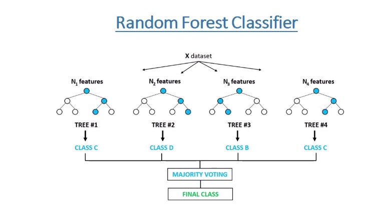
Tin Kam Ho introduced the general concept of Random Forests in the year 1995. It is an ensemble classification technique that has high accuracy. The error for classification decreases as the number of trees in the forest increases. Leo Breiman further established random forests more concretely in 2001, he defined random forests as a classifier that consists of a set of tree-based classifiers where each classifier has independent weights and independently casts votes for the most popular class of the data provided.
Advantages of Random Forests include:
- Reduces overfitting to a large extent.
- Works on both classification as well as regression problems.
- Normalization of data is unessential because of the rule-based approach.
- Has better accuracy as compared to decision trees
Disadvantages of Random Forests include:
- The process of training is computational expensive due to the large number of decision trees present.
- Time required for training is more when compared to decision trees.
Random Forest Classifier

ROC of Random Forest Classifier of training, testing and validation
To overcome the issue of linear boundary generation for non-linear data, we use the Random Forest Classifier, a non-linear classifier. In this case, we also see that the model overfits the data, possibly due to producing exact non-linear boundaries for classification. Tuning of Hyperparameters in the RF classifier affects all the decision trees, so one needs to find the tradeoff between the value of the ROC AUC metric obtained and the changes in the hyperparameters.

MCC of the random and scaffold split for training, testing and validation
The scaffold split train dataset has a higher MCC due to overfitting, whereas the random split model generalizes better. The scaffold split doesn’t generalize well on unseen data as the test and the validation set contains drugs with scaffolds different from the training set.
XGBoost Classifier
Chen and Guestrin from the University of Washington introduced XGBoost in the year 2016. XGBoost is an ensemble learning technique based on decision trees. While there do exist gradient boosting algorithms, none of them are as widely used as XGBoost due to it’s scalability, and it’s execution time, it is computationally very quick. XGBoost is known to achieve high accuracy on tabular data. It has the same advantages as random forest with the added advantage that it is quicker. XGBoost optimizes the algorithm to produce such low computational speed and high accuracy.
Some features of XGBoost include:
- Gradient-based Tree Boosting with L1/L2 Regularization.
- Construction of parallization on CPU cores.
- Distributed training on a cluster of machines for a large dataset.
- Out-of-Core computation for large datasets that cause storage problems.

AUC - ROC of XGBoost Classifier of training, testing and validation
The XGBoost model can overcome the problem of overfitting to a certain extent, as evident by the ROC AUC values of the training, testing, and validation datasets. Even the MCC metric values indicate that there is not much difference between the training, testing, and validation results obtained.

MCC of the random and scaffold split for training, testing and validation
Discussion
Some potential reasons for values of these metrics being moderate and not higher include -
- 1024 number of bits for the representation of drug molecules don’t fully capture the structure of molecules.
- The ECFP radii as 2 are not able to properly represent the molecule.
- Maybe the ECFP doesn’t adequately represent the molecules and a different molecular descriptor like Avalon Fingerprints, 2D Pharmacophore Fingerprints, etc.
Future Work
Future work includes:
- Further Evaluation of the results utilizing chemical space analysis on the predicted values and comparing the same to actual results to understand which particular molecule affects the model.
- Implementation of Deep Learning-based techniques such as Graph Convolutional Neural Networks and Multilayer Perceptron (MLP).
- Implementation of different descriptors for the drugs.
Code
The code for the project is available here.
References
- Tropsha, Alexander. “Best practices for QSAR model development, validation, and exploitation.” Molecular informatics 29.6‐7 (2010): 476-488
- Holmer, Malte, et al. “CYPstrate: A Set of Machine Learning Models for the Accurate Classification of Cytochrome P450 Enzyme Substrates and Non-Substrates.” Molecules 26.15 (2021): 4678
- Göller, Andreas H., et al. “Bayer’s in silico ADMET platform: A journey of machine learning over the past two decades.” Drug Discovery Today 25.9 (2020): 1702-1709
- Dataset
- Ho, Tin Kam. “Random decision forests.” Proceedings of 3rd international conference on document analysis and recognition. Vol. 1. IEEE, 1995
- Chen, Tianqi, and Carlos Guestrin. “Xgboost: A scalable tree boosting system.” Proceedings of the 22nd acm sigkdd international conference on knowledge discovery and data mining. 2016